Emulation Layer architecture

The ML Emulation Layer for Vulkan® implements ML extensions using Vulkan® compute. The graph layer turns graph operations into compute pipelines; the tensor layer represents tensor data with buffers and translates tensor accesses in compute shaders into buffer accesses. The underlying Vulkan® implementation executes the resulting commands.

Graph pipeline creation prepares reusable compute state. A graph session provides intermediate tensors and their memory bindings for execution. The application supplies external resources, records graph dispatches, and submits the command buffer through the usual Vulkan® APIs.

The ML Extension Overview page lists supported extensions and instruction sets; Data Graph and Tensors describe their API surfaces. See Usage for layer configuration and Known Limitations for platform constraints.

Layer integration

The tensor layer, VK_LAYER_ML_Tensor_Emulation, implements VK_ARM_tensors. It provides tensor objects, views, queries, memory binding, and tensor-aware compute shader processing. Applications can use this layer on its own for tensor compute workloads.

The graph layer, VK_LAYER_ML_Graph_Emulation, implements VK_ARM_data_graph and its TOSA and optical-flow extensions. Graph SPIR-V™ processing handles the supported TOSA and Motion Engine instruction sets; optical flow has a distinct internal implementation behind the same graph API. The graph layer creates compute execution structures and records commands for graph dispatches. It requires VK_LAYER_ML_Tensor_Emulation and the synchronization2 feature. The current implementation also requires the underlying device to advertise VK_KHR_synchronization2, even on Vulkan® 1.3 devices. The layer checks for this extension and adds it to the forwarded device-extension list during device creation.

Neither layer converts framework models, such as PyTorch or TensorFlow models, or reads VGF containers. Conversion and container decoding happen before the application submits Vulkan® workloads. The layers implement the Vulkan® APIs defined by their extensions and intercept supporting core Vulkan® calls; the application does not call a separate emulation-specific execution API. Native ML extension support is not required from the underlying implementation for the functionality supplied by the enabled layers.

Loader integration

Each layer is a shared library with a Vulkan® layer manifest. The loader uses these manifests to discover the layer names and libraries. Enabling a layer in the instance creation configuration, or through the loader’s environment configuration, asks the loader to insert it into the application’s Vulkan® call chain. Applications use the same Vulkan® commands and structures as they would with native extension support; enabling emulation does not change how they call those APIs.

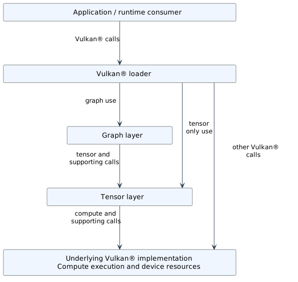
Graph emulation uses tensor emulation below it. Calls can also reach tensor emulation or the underlying implementation directly.

Enable the graph layer before the tensor layer when both are used. In this order, tensor API calls made by graph emulation reach tensor emulation below it. For direct tensor compute, enabling the tensor layer is sufficient; both layers can also remain enabled. See Usage for the configuration details.

Applications and the loader obtain Vulkan® command function pointers through vkGetInstanceProcAddr and vkGetDeviceProcAddr. Each layer provides implementations of these lookup functions, returning its own handlers for commands it intercepts. These include its extension commands and supporting Vulkan® commands for object creation, descriptor updates, and command recording. Commands that a layer does not intercept are resolved through the next layer or the underlying implementation. The diagram shows representative paths through this call chain.

Shared layer infrastructure maintains instance and device dispatch state and tracks associated queues and command buffers. Graph and tensor implementations add their own object state and interception behavior. Calls to lower layers use the next dispatch functions, allowing emulated operations to be implemented with underlying Vulkan® resources and compute commands.

Capabilities and device creation

Treat the Vulkan® implementation exposed through the enabled layers as the target implementation: query its capabilities and follow the same API contracts as for a device providing the extensions natively. Enable the layers before querying support, then select the required extensions, features, formats, and queues. Create the device, resources, pipelines, and graph sessions required by that workload. Follow Usage for layer configuration and Known Limitations when selecting a workload or investigating unsupported behavior.

The layers augment device-extension enumeration and intercept the relevant feature, property, and format queries. Some reported capabilities are supplied by emulation; others are derived from the underlying implementation. For example, the graph layer adds the data-graph queue flag to queue families that support compute. Tensor limits and optional descriptor-indexing features are constrained by the underlying buffer and descriptor capabilities.

Applications must also query operation-specific support. Graph execution, TOSA instruction sets, optical flow, and tensor shader access have different constraints; advertising an extension name alone does not establish that a particular combination of operations, data types, and resource formats will work. The detailed query surfaces are listed in Data Graph and Tensors.

At device creation, the layers adapt the requested extension and feature structures for the next implementation. Shared infrastructure removes layer-implemented extension names from the forwarded extension list and adds required lower-level extensions. The layer implementations consume their ML feature structures and translate applicable feature requests into underlying requirements. This lets an application request emulated ML functionality without asking the driver to implement those extension names itself.

The underlying implementation still executes the compute work and provides memory, queues, and the other Vulkan® capabilities required by that work. Enabling a layer does not supply every optional feature or make every workload supported. The current device-creation path requires Vulkan® 1.3 when a layer-provided ML extension is enabled.

Tensor emulation

Tensor emulation supplies the storage and shader-access model used by both direct tensor compute and the graph layer’s generated compute workloads.

Buffer-backed tensor data

Internally, TensorARM creates a VkBuffer for the tensor elements. vkBindTensorMemoryARM binds that buffer to the supplied VkDeviceMemory and offset. A tensor view refers to this tensor and provides the descriptor representation used when binding it to a shader.

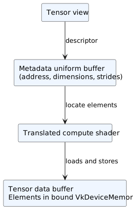
Tensor metadata and element storage are separate buffers. Shader accesses use metadata to locate elements in the bound data memory.

Tensor descriptors are backed by small uniform buffers containing the tensor data address, dimensions, and strides. They describe the elements; the elements themselves remain in the tensor’s storage buffer. The translated shader uses that metadata to calculate element offsets and perform buffer loads and stores. The usual address-based path uses buffer device addresses, while the MoltenVK compatibility path can use additional storage-buffer descriptor bindings for the same tensor data.

Creating a tensor creates a buffer object but does not allocate memory for its elements. The caller supplies and binds the VkDeviceMemory allocation. Tensor views have small metadata buffers allocated by the tensor layer; these do not take ownership of the element allocations. Passing a tensor between compute stages uses the bound data in place and does not imply a host copy per dispatch. Graph constants and intermediate tensor storage are described in Pipeline and session state.

Tensor shader processing

Tensor-aware compute shaders can be supplied by an application or created by the graph layer. In both cases, tensor emulation translates their tensor instructions into buffer accesses before the underlying implementation creates the compute pipeline.

The default translation path uses SPIRV-Cross to emit GLSL and glslang to compile it back to SPIR-V™. The experimental direct SPIR-V™ path, selected with VMEL_EXPERIMENTAL_TENSOR_LOWERING_MODE=1, performs the supported lowering without that GLSL round trip.

Graph pipeline construction

The following flows describe graph SPIR-V™ using supported instruction sets. Optical-flow single-node pipelines enter through the same creation API but select a separate implementation; they do not run the SPIR-V™ graph-processing pass shown here. See Data Graph for the supported paths and API surface.

An application supplies a graph module, constant data, and resource metadata through VkDataGraphPipelineCreateInfoARM, its pResourceInfos array, and associated pNext structures. Descriptor set layouts and a pipeline layout describe the graph’s external interface. Resource metadata supplies the tensor format, dimensions, and strides for each descriptor set, binding, and array element; the application binds the actual input and output resources later.

vkCreateDataGraphPipelinesARM selects the graph or optical-flow path from its creation structures. For a graph, the shader-module creation structure provides constants identified by integer IDs and the module to process. The implementation accepts a graph shader-module handle created through its intercepted vkCreateShaderModule or inline SPIR-V™ in a VkShaderModuleCreateInfo on the creation chain. It copies resource descriptions into internal tensor metadata and initializes pipeline-owned constant tensors from the supplied data.

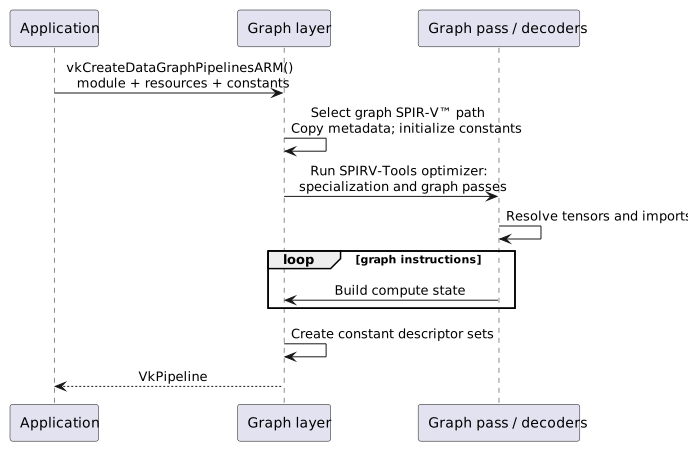
Construction of a pipeline from graph SPIR-V™. API creation structures supply inputs used to build internal compute state.

During vkCreateDataGraphPipelinesARM, the graph layer checks the module’s extended instruction-set imports and creates a SPIRV-Tools Optimizer. It registers any required specialization-constant processing passes followed by GraphPassExtInst, then calls Optimizer::Run on the supplied SPIR-V™. A shared graph context resolves constants and input/output tensors. The instruction-set registry selects the TOSA or Motion Engine decoder for each extended instruction import, and the decoder builds the corresponding compute operations.

The resulting GraphPipeline retains ordered compute operations, their internal layouts, tensor metadata, and constants. Compute implementations use embedded shader variants and the supplied Vulkan® pipeline cache handle where applicable. Graph processing constructs execution state as a side effect of the pass; the optimizer’s output module is not the graph’s execution product. The layer copies the metadata and constant data it needs into this internal state. The application follows the Vulkan® lifetime rules for its original objects and input structures.

Shader generation and selection

The graph layer implements supported TOSA and Motion Engine operations as separate compute workloads. Instruction-set decoders resolve each operation’s input/output tensors and attributes, then call the corresponding GraphPipeline factory. The factory constructs compute implementation objects with an internal descriptor layout, shader module, and compute pipeline. Those objects become the graph’s ordered execution stages.

The graph kernels are authored as GLSL templates under graph/shaders/graph_op. During the layer build, CMake combines each kernel with shared GLSL support, substitutes arithmetic/storage types and other variant definitions, and invokes glslang to produce tensor-aware SPIR-V™. Generated C++ arrays and a shader registry embed those binaries in the layer. The installed library therefore carries its graph kernel variants.

At graph pipeline creation, each compute implementation selects an embedded variant through PipelineCache::lookup, supplies applicable specialization constants, and retains push-constant data for later command recording. The lookup is an embedded shader registry; the Vulkan® pipeline cache handle is separately passed to compute pipeline creation. Runtime selection does not regenerate the graph’s GLSL templates.

The selected binaries still contain tensor instructions. The tensor layer translates these as described in Tensor shader processing; compiling graph templates during the build and translating tensor instructions during pipeline creation are distinct steps.

Operator emulation with compute shaders

TOSA CONV2D illustrates how an operator becomes a compute workload. Its decoder resolves the input, weights, bias, and output tensors, then calls makeConv2D to construct a Conv2D implementation. The internal descriptor map binds these four tensors to the kernel. Input, weight, output, and accumulator arithmetic types select the embedded shader variant; padding, stride, dilation, and input/weight zero points are retained as push-constant data for command recording.

When the recorded workload executes, the convolution shader reads input and weight values, accumulates their products, adds the bias, and writes the output tensor. Its dispatch geometry comes from the output dimensions. If the work exceeds the device’s workgroup-count limits, Conv2D records several dispatches with output-position offsets identifying each portion of the work.

Some other TOSA operations illustrate different compute patterns:

• REDUCE_SUM uses the shared Reduce implementation, selecting a shader variant for summation and the input tensor’s arithmetic type. Tensor rank is a specialization constant, and the reduction axis is push-constant data. Each shader invocation computes an output element by reading and summing input elements along that axis.

• CONCAT creates a Concat compute stage for each input tensor. The stages share the output tensor, with the concatenation axis and a cumulative output offset supplied as push constants. Each stage copies its input elements into the corresponding region of the output tensor.

Motion Engine’s sum-of-absolute-differences operations use the same compute infrastructure through BlockMatch. Its shader variants write best-match vectors (MIN_SAD), vectors and costs (MIN_SAD_COST), or candidate costs (RAW_SAD). Kernel and search geometry become specialization constants.

These examples show why stage and dispatch counts can differ from graph operation counts. Structural graph instructions such as composite-result extraction resolve tensor references without adding another compute kernel. The resulting compute stages are retained by the graph pipeline; recording them for execution requires a session and bound resources.

Graph execution

Executing a prepared graph connects its reusable compute state to session memory and application resources before recording commands.

Pipeline and session state

A graph pipeline contains reusable compute state and constant tensors. Each DataGraphPipelineSessionARM retains a shared reference to that pipeline and creates its own intermediate tensor instances, descriptor sets, and memory planner. The pipeline describes the intermediates; the session instantiates their storage bindings.

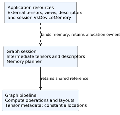
Internal graph state and application resources. Solid arrows describe retained or owned state; the dashed memory link represents binding without allocation ownership.

Pipeline constant allocations are created and initialized by the library and released with the internal graph pipeline. Session tensor objects and descriptors are managed by the session, but the application allocates the VkDeviceMemory used for session intermediates. Binding that memory does not transfer allocation ownership. External input/output tensors, their views, and their memory likewise remain application resources.

The internal shared reference explains how sessions reach compiled state; it does not relax public object-lifetime or synchronization requirements. The application must keep resources and bound memory valid while recorded work can use them, complete that work before releasing them, and destroy its public objects according to the API contracts.

Session memory preparation

Session creation constructs intermediate descriptors and a memory plan. The default IntervalMemoryPlanner derives tensor live intervals from compute execution order and tensor dependencies, then assigns aligned offsets. Tensors whose live intervals do not overlap can reuse memory; the requirement is therefore not simply the sum of all intermediate tensor sizes. Tensors for which no live interval was inferred are handled conservatively by the planner. Set VMEL_MEMORY_PLANNER to Linear or BestFit to select an alternative planner. If the variable is unset or has any other value, the interval planner is used.

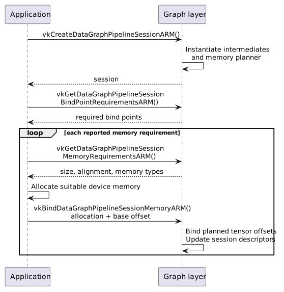
Session creation, requirement queries, allocation, and binding for graphs using SPIR-V™ extended instructions.

The application first enumerates bind-point requirements with vkGetDataGraphPipelineSessionBindPointRequirementsARM. The SPIR-V™ graph path reports a transient memory bind point when its planned size is nonzero; a graph needing no intermediate memory can report no bind points. For each reported requirement, the application queries vkGetDataGraphPipelineSessionMemoryRequirementsARM and chooses memory satisfying its size, alignment, and memory-type constraints.

vkBindDataGraphPipelineSessionMemoryARM supplies the allocation and base offset. The planner binds each intermediate at its assigned offset relative to that base, and the layer updates the session’s compute descriptors. Constants and external tensors are outside this transient allocation. Optical-flow sessions can also report an optical-flow cache bind point when requested; that lifecycle is separate from the SPIR-V™ graph flow described here.

Descriptor mapping and dispatch

Application descriptor sets express graph bindings. Tensor descriptor writes use VkWriteDescriptorSetTensorARM to supply tensor views; the graph layer tracks those views by descriptor binding and by index within that binding’s application descriptor array. VkWriteDescriptorSet.dstArrayElement selects the first array entry being written, and VkWriteDescriptorSetTensorARM.pTensorViews supplies the views for consecutive entries. For example, a write with dstArrayElement = 2 and one tensor view updates element 2 of that binding. The layer’s compute implementations have their own pipeline layouts and descriptor coordinates. A single graph resource may therefore feed multiple internal compute bindings.

On first use for a graph pipeline and graph set, the layer creates the required external compute descriptor sets and resolves the tracked tensor views into them. These mappings are cached on the tracked application descriptor set by graph pipeline and set; subsequent descriptor writes update existing mappings. Using update-after-bind descriptors with a graph pipeline requires the dataGraphUpdateAfterBind feature and the appropriate update-after-bind descriptor flags. Vulkan® resource lifetime and synchronization rules still apply.

Command recording and submission

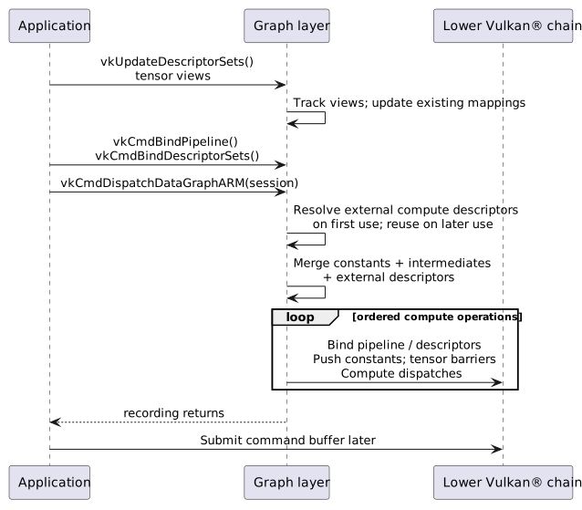
Recording a graph dispatch resolves graph resources into internal compute descriptors. Submission remains with the application.

At vkCmdDispatchDataGraphARM, the session identifies the graph pipeline. The layer combines three descriptor maps: pipeline constants, session intermediates, and application external resources. Map entries are keyed by internal compute pipeline layout and descriptor set, allowing each operation to retrieve its own bindings.

The pipeline then walks its ordered compute operations. Their recording path binds compute pipelines and descriptors, pushes applicable constants, inserts tensor dependency barriers for inputs, and records compute dispatches. The tensor layer translates the tensor operations and supporting calls to the underlying implementation. This happens while recording the application’s command buffer; graph dispatch does not submit that buffer or wait for it.

The application controls submission, completion, and synchronization with uploads, downloads, and other rendering or compute work. Internal graph barriers handle the emulated operations’ dependencies and do not establish all dependencies with surrounding application work.